library(rgbif)Occurrence Records
Overview
- Retrieve occurrence records for Bombus sitkensis from the Global Biodiversity Information Facility (GBIF)
- Process these records along with the environmental rasters to create presence and background points to use for fitting the species distribution model
1. Use rgbif to get occurrence records
The package rgbif enables you to access GBIF’s API and request records downloads. Download requests are associated with a DOI, making them reproducible and citeable.
Load the package
Set up GBIF credentials
To download from GBIF, you need to register and supply your registration credentials. More on this here. Or you can use the account info that we’ve provided for this workshop.
Once you have your credentials ready, you need to add them to your R environment. The package usethis has a handy function that brings up the file you need to edit to do this:
library(usethis)

usethis::edit_r_environ()
This will bring up a file called .Renviron. Replace your own credential information below (replace the info in quotes with your info), or you can use the account info that we will provide for this workshop. Then, copy this information into the .Renviron file and save it.
GBIF_USER="your_username"

GBIF_PWD="your_password"

GBIF_EMAIL="youremail@gbif.org"
After changing the .Renviron file, you must restart your R session by running the code below.
.rs.restartR()Or, in the Rstudio menu, go to Session > Restart R. If you use the menu option, make sure to reload the rgbif package using library(rgbif).
Get the GBIF taxon key
Although we can search GBIF using the scientific name, this can sometimes return poorly matched results if things like authorship information are missing. We can use the function rgbif::name_backbone() to identify the GBIF taxon key that will return precise taxon matches.
name_backbone("Bombus sitkensis")# A tibble: 1 × 22
usageKey scientificName canonicalName rank status confidence matchType
* <int> <chr> <chr> <chr> <chr> <int> <chr>
1 1340328 Bombus sitkensis Nyl… Bombus sitke… SPEC… ACCEP… 97 EXACT
# ℹ 15 more variables: kingdom <chr>, phylum <chr>, order <chr>, family <chr>,
# genus <chr>, species <chr>, kingdomKey <int>, phylumKey <int>,
# classKey <int>, orderKey <int>, familyKey <int>, genusKey <int>,
# speciesKey <int>, class <chr>, verbatim_name <chr>The taxon key for Bombus sitkensis is 1340328.
Set up an rgbif query
There are many query parameters available to narrow down a request for observation records. We are including a few parameters that indicate acceptable-quality data for creating robust distribution maps. These include:
- Has geographic coordinates
- Has no geospatial issues
- Has acceptable geospatial coordinate accuracy
- Represents the presence of the target organism
- Within a desired time range
- Represents a human observation
- Is within our focal geographic extent
The GBIF API has specific search terms (called ‘predicates’ in their domain-specific language) that can specify these parameters. Below we are creating variables to store these values
# has geographic coordinates
hasCoordinate <- TRUE

# has no geospatial issues
hasGeospatialIssue <- FALSE

# acceptable geospatial coordinate accuracy: from 0 to 120 m accuracy
coordinateUncertaintyInMeters <- "0,120"

# occurrence status should be "PRESENT"
occurrenceStatus <- "PRESENT"

# time range is from 2015 to 2025
year <- "2015,2025"

# type of record is human observation
basisOfRecord <- "HUMAN_OBSERVATION"

# define the geographic extent
stateProvince <- "Oregon"
country <- "US"
Now we can use the function rgbif::occ_count() to preview how many GBIF records we will return if we use these search terms.
occ_count(
  taxonKey = 1340328,
  hasCoordinate = hasCoordinate,
  hasGeospatialIssue = hasGeospatialIssue,
  coordinateUncertaintyInMeters = coordinateUncertaintyInMeters,
  occurrenceStatus = occurrenceStatus,
  year = year,
  basisOfRecord = basisOfRecord,
  stateProvince = stateProvince,
  country = country
)
[1] 204Make the GBIF request
Now that we know everything works, we make an actual request. We can use the function occ_download() to actually get the data.
gbif_download <- occ_download(
  pred("taxonKey", 1340328),
  pred("hasCoordinate", hasCoordinate),
  pred("hasGeospatialIssue", hasGeospatialIssue),
  pred_lte("coordinateUncertaintyInMeters",120),
  pred_gte("coordinateUncertaintyInMeters",0),
  pred("occurrenceStatus", occurrenceStatus),
  pred_gte("year", 2015),
  pred_lte("year", 2025),
  pred_in("basisOfRecord",basisOfRecord),
  pred("country", country),
  pred("stateProvince",stateProvince)
)
Note that the syntax is different from the occ_search() function. It makes use of pred* functions that define the filters we are defining using our search term variables from above. The first argument in is a key defining the filter, followed by the value.
For example,
pred("taxonKey", 1340328)filters for records withtaxonKey1340328, andpred("hasCoordinate", hasCoordinate)filters for records withhasCoordinatevalues equal to what we defined for the variable with the same name, abovepred_lte("coordinateUncertaintyInMeters",120)andpred_gte("coordinateUncertaintyInMeters",0)indicate that the keycoordinateUncertaintyInMetersshould be “less than or equal to 120” and “greater than or equal to 0”Similarly,
pred_gte("year", 2015)andpred_lte("year", 2025)indicateyearshould be >= 2014 and <= 2025
We can check on the status of the download by running the download object:
occ_download_wait(gbif_download)Example output, once the download has succeeded:
<<gbif download metadata>>
  Status: SUCCEEDED
  DOI: 10.15468/dl.w593th
  Format: DWCA
    Download key: 0013939-251025141854904
  Created: 2025-11-03T22:09:31.716+00:00
  Modified: 2025-11-03T22:11:28.499+00:00
  Download link: https://api.gbif.org/v1/occurrence/download/request/0013939-251025141854904.zip
  Total records: 204
Once the download is ready, we can get the data:
occ <- occ_download_get(gbif_download) |> occ_download_import()Citing the download
We can get a citation with a doi, using the gbif_citation function and a Download key from the gbif_download object. An the example from the output above:
gbif_citation("0013939-251025141854904")$download
[1] "GBIF Occurrence Download https://doi.org/10.15468/dl.w593th Accessed from R via rgbif (https://github.com/ropensci/rgbif) on 2025-11-03"
$datasets
NULL2. Process occurrence data
Load environmental and habitat rasters
The following steps require the library terra and the environmental and habitat layers from the last section. Load these if you don’t have them in your environment already.
library(terra)

prmean <- rast("data/prmean.tif")
tmean_yr <- rast("data/tmean_yr.tif")
tmax_yr <- rast("data/tmax_yr.tif")
tmin_yr <- rast("data/tmin_yr.tif")
elevcc <- rast("data/elevcc.tif")
forageFall <- rast("data/forageFall.tif")
forageSpring <- rast("data/forageSpring.tif")
forageSummer <- rast("data/forageSummer.tif")
nesting <- rast("data/nesting.tif")
insecticide <- rast("data/insecticide.tif")
Rename rasters
When making these rasters, the terra package automatically generates names that aren’t always legible. Here we use the names() <- function to rename the layers to something more understandable.
# rename layers for reference

names(prmean) <- "prmean"
names(tmean_yr) <- "tmean"
names(tmax_yr) <- "tmax"
names(tmin_yr) <- "tmin"
names(elevcc) <- c("elev", "canopycov")
names(forageSpring) <- "forageSpring"
names(forageSummer) <- "forageSummer"
names(forageFall) <- "forageFall"
names(nesting) <- "nesting"
names(insecticide) <- "insecticide"
Create occurrence grid for Bombus sitkensis
We use the coordinates of the GBIF observations to convert into georeferenced points using the vect function in terra.
occ.vect <- vect(occ[,c("decimalLongitude","decimalLatitude")],
                 geom = c("decimalLongitude","decimalLatitude"), # x and y columns
                 crs = "epsg:4326")  # WGS 1984 geographic coordinate system

plot(occ.vect)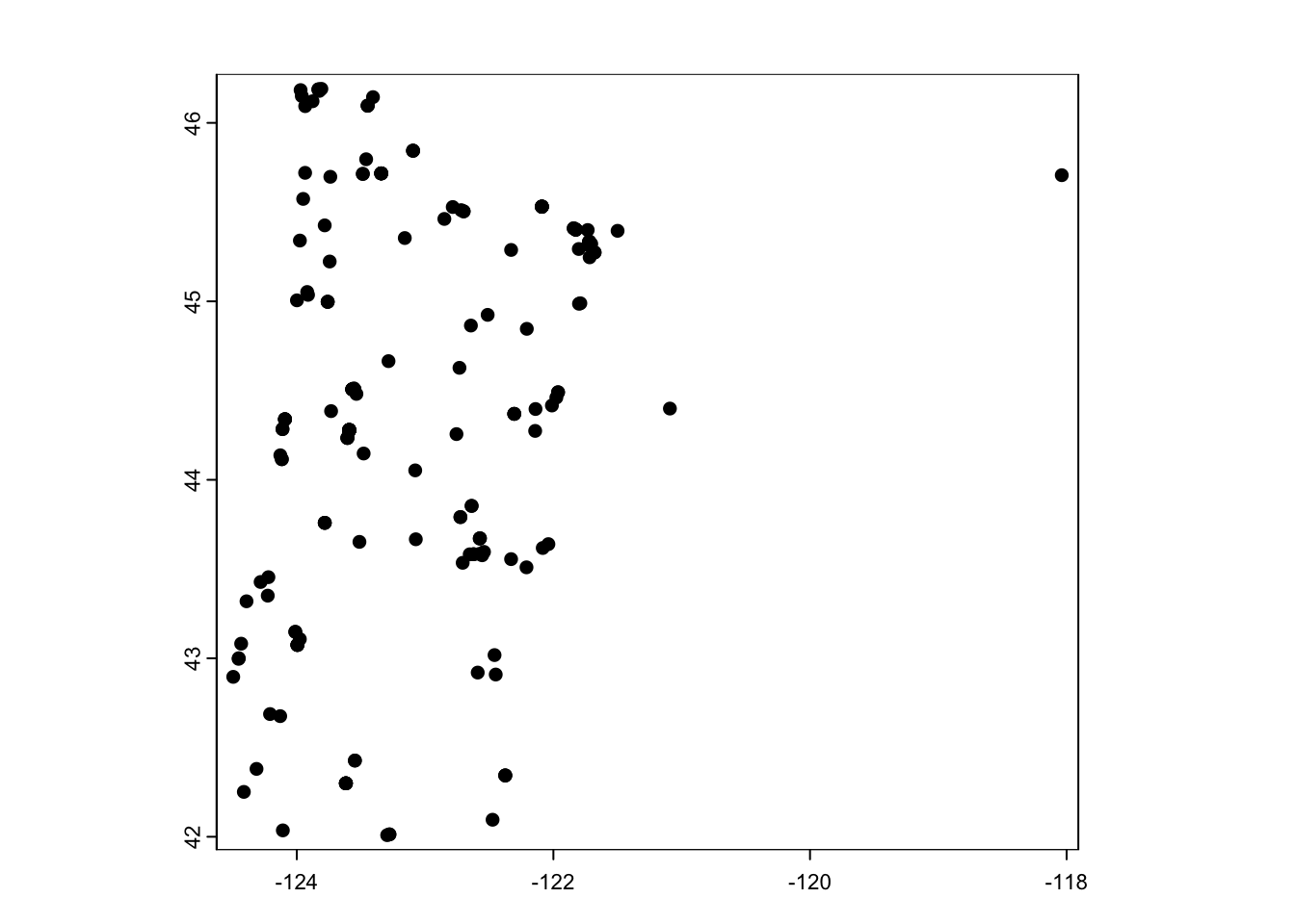
Convert the observed points to grid cells
Using one of the environmental grids as a template, we convert the observation points from GBIF to a presence grid, where a grid cell value of 1 indicates that (any number of) observations were reported in that cell.
occ.rast <- rasterize(occ.vect |>
                        terra::project(prmean),   # project points to match projection
                      prmean                      # template raster
                      )

# rename the raster layers for reference

names(occ.rast) <- "B_sitkensis"

plot(occ.rast, col = "blue")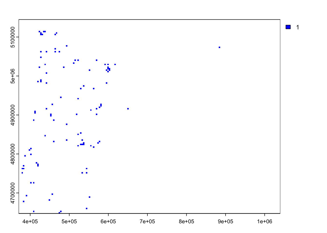
Combine presence grid with environment and habitat variables and extract to table
We only need a table of presence grid cells and their associated habitat and environmental values. To do this, we can stack all the raster layers together (since they share the same projection and their grids are aligned). Then we can use the terra values function to extract the cell values of the stacked grids as rows in a table, keeping only the rows with B. sitkensis presences using the filter function from dplyr.
library(dplyr)

# stack then environmental and habitat layers and the rasterized occurence points

occ.envr <- rast(list(prmean, tmean_yr, tmax_yr, tmin_yr, elevcc, forageFall,
                      forageSpring, forageSummer, nesting, insecticide, occ.rast))


presence <- as.data.frame(occ.envr, xy = TRUE) |>
  na.omit()   # drop rows where B_sitkensis occurence is NA
Create background points grid
Background samples are obtained randomly and independently of species locations. Background points are meant to sample the full environmental space available to the species of interest in the region. This means that background points:
- should be numerous enough to represent the environmental variation across the region
- may overlap with the presence points
The package predicts has a function that is useful for creating background points, backgroundSample.
library(predicts)

set.seed(100)   # background sampling is random. Setting seed to 100 ensures we get the same results

backgroundpts <- backgroundSample(
  mask = forageFall,           # mask restricts points to area of interest (defined by the forageFall)
  n = 10000,                   # create 10000 background points
)

background <- terra::extract(occ.envr[[1:11]],    # only extracting the environmental/habitat layers
                      backgroundpts               # extraction locations
                      )

# combine presence and background data

presback <- bind_rows(presence, background) |>
  mutate(B_sitkensis = ifelse(is.na(B_sitkensis), 0, B_sitkensis))   # replace NA (from background data) with 0
Save the output!
saveRDS(presback, "data/presback.rds")
saveRDS(occ.envr, "data/occ.envr.rds")